LSD direction vectors
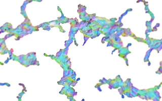
Direction vectors of the LSDs on a single neuron from the fly visual system. Colors correspond to the direction in which the neuronal processes travel.

Local Shape Descriptors for Neuron Segmentation

Abstract

We present a simple, yet effective, auxiliary learning task for the problem of neuron segmentation in electron microscopy volumes. The auxiliary task consists of the prediction of Local Shape Descriptors (LSDs), which we combine with conventional voxel-wise direct neighbor affinities for neuron boundary detection. The shape descriptors are designed to capture local statistics about the neuron to be segmented, such as diameter, elongation, and direction. On a large study comparing several existing methods across various specimen, imaging techniques, and resolutions, we find that auxiliary learning of LSDs consistently increases segmentation accuracy of affinity-based methods over a range of metrics. Furthermore, the addition of LSDs promotes affinity-based segmentation methods to be on par with the current state of the art for neuron segmentation (Flood-Filling Networks, FFN), while being two orders of magnitudes more efficient - a critical requirement for the processing of future petabyte-sized datasets. Implementations of the new auxiliary learning task, network architectures, training, prediction, and evaluation code, as well as the datasets used in this study are publicly available as a benchmark for future method contributions.


Contents

Tl;dr


Background

Connectomics

Connectomics is an emerging field which integrates multiple domains including neuroscience, microscopy, and computer science. The overarching goal is to provide insights about the brain at resolutions which are not achievable with other approaches. The ability to study neural structures at this scale will hopefully lead to a better understanding of brain disorders, and subsequently advance medical approaches towards finding treatments & cures.

The basic idea is to produce "connectomes" which are essentially maps of the brain. These maps, or "wiring diagrams", give scientists the ability to see how every neuron interacts through synaptic connections. They can be used to complement existing techniques and drive future experiments .

Currently, only Electron Microscopy (EM) allows imaging of neural tissue at a resolution sufficient to see individual synapses. Unfortunately, by imaging brains at such high resolution, the resulting data is massive. Let's consider a fruit fly example. A full adult fruit fly brain (FAFB) imaged with ssTEM at a pixel resolution of ~4 nanometers and ~40 nanometer thick sections, comprises ~50 teravoxels of data (neuropil). For reference, a voxel is a volumetric pixel, and the "tera" prefix means 1012. So, one fly brain contains upwards of 50,000,000,000,000 volumetric pixels. To put that in perspective, Abbott et al. argue that, assuming a scale where 1000 cubic microns is equivalent to 1 centimeter, a fruit fly brain would comprise the length of 6 and a half Boeing 747 aeroplanes. This still pales in comparison to a mouse brain which would require the acquisition of 1 million terabytes of data.

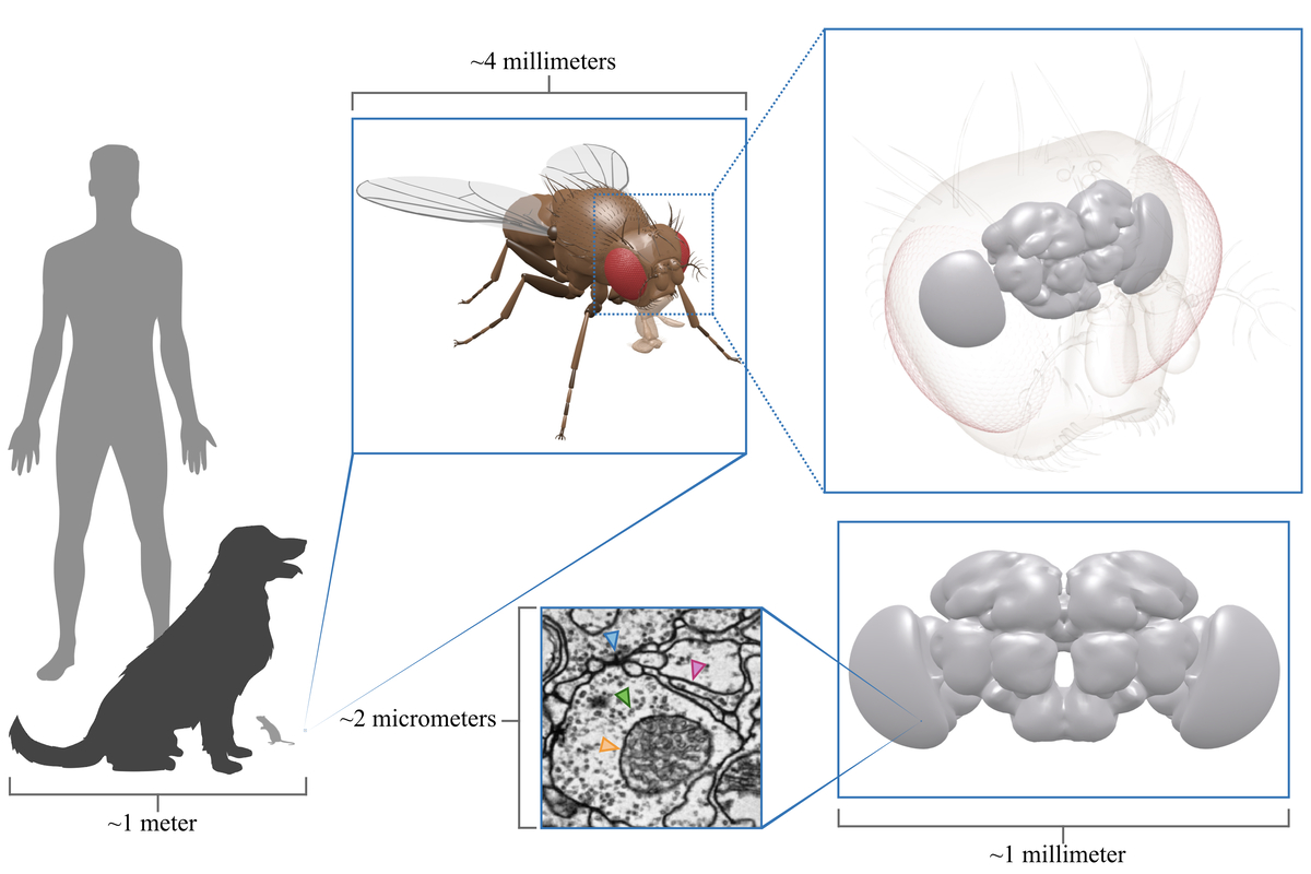
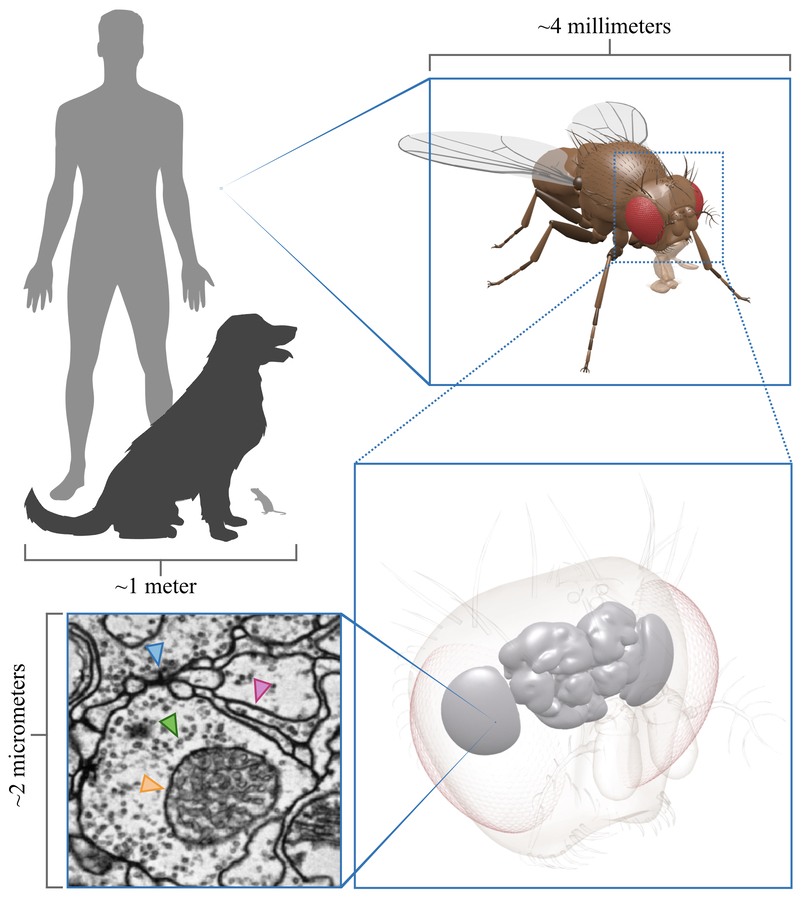
Scale perspective. A fruit fly brain imaged at synaptic resolution takes up 100's of terabytes of storage space. It allows us to see fine structures such as neural plasma membranes (pink arrow), synapses (blue arrow), vesicles (green arrow) and mitochondria (orange arrow). 3D fruit fly model kindly provided by Igor Siwanowicz

Okay, now we have the data, so how do we create the wiring diagrams?

To create a wiring diagram, we need to reconstruct all of the neurons and their synaptic connections. This process can be done manually - which consists of human annotators navigating these datasets and labeling every neuron and their synaptic partners using various software . However, this can become extremely tedious and expensive ($$$) given the size of the datasets. For example, simply reconstructing 129 neurons from FAFB took a team of tracers ~60 days to complete. Given that a fruit fly has ~100,000 neurons, purely manual reconstruction of connectomes is obviously infeasible.

Consequently, methods have been developed to automate this process. From here on, we will focus on the automatic reconstruction of neurons. To see the current approaches to synapse detection, check these papers out!

Neuron Segmentation

Neuron segmentation is the current rate-limiting step for generating large connectomes. Errors in a neuron segmentation can easily propagate throughout a dataset as the scale increases, which makes it tedious for humans to proofread the data without advanced tools.

Neuron reconstruction is an instance segmentation problem because every pixel of every neuron needs to be assigned a unique label (in contrast to object detection and semantic segmentation). Take the following example:

Given a raw EM image, we could simply detect mitochondria (object detection), assign all pixels containing mitochondria to one class (semantic segmentation), or assign all pixels of each object to a unique class (instance segmentation). Our goal in this paper is the latter.

It would be ideal to directly predict unique labels (i.e neurons) in a dataset. Unfortunately this requires global information which is difficult because neurons span large distances. Due to the nature of neural networks, field of views are not large enough to account for downstream changes in a neuron such as branching and merging. Consequently, alternative approaches aim to solve the problem locally.

Most current approaches to neuron segmentation center around producing boundary maps which are then used to generate unique objects with post-processing steps. Consider the following example:

We have four neurons (A,B,C,D) and we want to assign voxels (squares) to the label they belong to. Images kindly provided by Stephan Saalfeld.
Naively labeling foreground voxels (white squares) and background voxels (black squares) would result in the top part of the yellow neuron (B) being falsely labeled as background.
The top part of the yellow neuron would now be correctly assigned. However, slight changes in boundary predictions could result in subsequent post-processing errors.
Several increased neighborhood steps can be used to provide increased context to the nearest neighbor affinities. This essentially allows the network to see more than it otherwise would.
After predicting affinities, losses are computed on maximin edges and a maximal spanning tree (line) is grown to identify maximin edges.
Given seed points inside a neuron (large white square, for example), the network predicts which voxels belong to the same neuron (white squares) and which belong to different neurons (black squares).

Contributions


Methods

Local Shape Descriptors

The intuition behind LSDs is to improve boundary detection by incorporating statistics describing the local shape of an object close to a boundary. A similar technique produced superior results over boundary detection alone . Given a raw EM dataset and unique neuron labels, we can compute ground truth LSDs in a local window. Specifically, for each voxel, we grow a gaussian with a fixed radius and intersect it with the underlying label. We then calculate the center of mass of the intersected region and compute several statistics between the given voxel and the center of mass. This is done for all voxels in the window. Perhaps the most important is the mean offset to center of mass (shown below). This component ensures that a smooth gradient is maintained within objects while providing sharp contrasts at object boundaries.

Given raw data and ground truth labels we can compute LSDs. The general idea is to grow a gaussian around each voxel and intersect it with the underlying label. The center of mass of the intersected region is calculated, and statistics between the voxel and center of mass are computed. Here we see the first component of the LSDs, the mean offset to center of mass. At object boundaries, vectors are sharply contrasted in opposing directions. As we get closer to the center of objects, the difference between the selected voxel and center of mass decreases, which results in a smoother gradient.

Additionally, we calculate two statistics describing the directionality of neural processes (Covariance and Pearson's correlation coefficient). The former highlights the orientation of neurons while the latter exposes elongation. The final component is simply the voxel count inside the intersected region which translates to the size of the process.

The components of the LSDs, offset to center of mass ([0:3]), covariance ([3:6]), Pearson's correlation coefficient ([6:9]), and voxel count ([9:10]). The covariance describes neuron orientation (blue = x direction, green = y direction, red = z direction), Pearson's describes elongation (or changes in the orientation), and voxel count describes the size of the object (blue = small, red = big).

Since the LSDs are predicted in three dimensional space, it can be more intuitive to visualize how they map to a reconstructed neuron. For example, the following shows a 3D mesh reconstruction of a neuron alongside the orientation component of the LSDs (LSDs[3:6]):

3D reconstruction of a segmented neuron (blue mesh), with the corresponding LSD direction vectors. The orientation of the neuron is directly mapped to RGB space. If the neuron is moving in the Z direction, it is visualized as red. The Y direction is mapped to green, and the X direction is mapped to blue. Intermediate directions are mapped to intermediate colors.

Network Architectures

We implemented the LSDs using three network architectures. All three networks use a 3D U-Net A type of Convolutional Neural Network (CNN) which has both a downsampling and upsampling path (giving it the shape of a "U"). The best performing architecture uses an auto-context approach. The first pass predicts LSDs directly from raw data:

The LSD network weights are then used to predict LSDs in a larger region. The predicted LSDs are fed into a second network (AcRLSD) along with raw data in order to predict affinities:

See the paper for details on the other two networks (MtLSD & AcLSD). After training the networks for a number of iterations (usually several hundred thousand), the predicted LSDs start to resemble the ground truth LSDs. For example, when considering the offset vectors, we can see sharp contrasts at object boundaries, and smooth gradients within objects:

Ground truth LSDs (left), and predicted LSDs (right). Label boundaries were slightly eroded to produce gaps in the ground truth LSDs between objects. This forces the network to guess what to predict in these regions.

Results

We conducted a large scale study comparing LSD-based methods against three previous affinity-based methods: (1) direct neighbor and (2) long-range affinities with mean squared error (MSE) loss, and (3) direct neighbor affinities with MALIS loss. We also include comparisons against single FFN segmentations. For a more detailed overview, see section 3.1 in the paper.

Datasets

We used three large and diverse EM datasets to evaluate all methods and compare metrics.

The main component of the study was a region taken from songbird neural tissue . The volume comprises ~106 cubic microns of raw data. It was imaged using SBFEM at 9x9x20 (xyx) nanometer resolution. 0.02% of the data was using for training (33 volumes containing ~200 cubic microns of labeled neurons). 12 manually traced skeletons (13.5 millimeters) were used for network validation and 50 skeletons (97 millimeters) were used for evaluation:

Zebrafinch dataset overview. 1. 33 gound truth volumes were used for training. 2. Full raw dataset, scale bar = 15 μm. 3. Single section shows ground-truth skeletons, zoom in scale bar = 500 nm. 4. Validation skeletons (n=12, 13.5 mm). 5. Testing skeletons (n=50, 97mm)

After training, we predicted in a slightly smaller testing region (~800,000 cubic microns) which we refer to as the Benchmark ROI (region of interest). We created two sets of supervoxels, one without any masking, and one constrained to a neuropil mask. For each affinity-based network, we created segmentations over a range of ROIs in order to assess performance with scale. We then evaluated VoI, ERL, and MCM. See the paper for details on the other two datasets.

Accuracy

We found that the LSDs are beneficial for improving the accuracy of direct neighbor affinities and subsequently the resulting neuron segmentations. On the Zebrafinch dataset, we found that LSD architectures out-perform other affinity-based networks over a range of ROIs when used in an auto-context approach. When considering segmentation performance restricted directly to neuropil, our best auto-context network (AcRLSD) performs on par with the current state of the art when considering VoI:

VoI Sum vs ROI size. Each point corresponds to an ROI size. It is ideal to minimize VoI Sum. As we scale up, VoI increases because the number of errors increase. The best LSD network (AcRLSD - orange) is competitive with FFN (black).

We did not find this to be the case when evaluating ERL, which could be a direct result of asymmetric contributions of split and merge errors in the metric. ERL can not exceed the average length of skeletons, and thus the addition of shorter skeletons fragments can result in a decrease of ERL, even in the absence of errors. ERL measures do not progress monotonically over RoI sizes and absolute values are likely not comparable across different dataset sizes:

ERL (nanometers) vs ROI size. As we scale up, we observe varying ERLs across all networks from cutting the ground truth skeletons. This makes it hard to deduce network accuracy from this metric when evaluating on cropped volumes.

Throughput

As described previously, the acquisition size of datasets is growing rapidly. Segmentation methods should complement this trajectory by being fast and computationally inexpensive. When considering computational costs in terms of floating point operations (FLOPs), we found that our best method (AcrLSD) is two orders of magnitude more efficient than the current state of the art, while producing segmentations of comparable quality:

Accuracy vs computational costs. Over a range of ROIs (points) affinity-based methods require significantly less teraFLOPs (floating point operations) than FFN. Auto-context networks (green/orange) are also accurate enough to make their slight computational overhead justifiable.

All affinity-based methods can be parallelized efficiently using a modest amount of GPUs, resulting in higher throughput:

Inference costs on Zebrafinch benchmark ROI (~800k cubic microns). Predicting LSDs, for example, took 2 hours using 100 GPUs.

This is accomplished using a block-wise processing scheme in which a large volume is broken down into smaller chunks. The chunks can then be distributed over many workers in such a way that ensures non-neighboring blocks are processed simultaneously. As soon as a worker finishes processing a block it will start processing another valid block. This repeats until the entire volume is processed. Consider watershed as an example:

Overview of block-wise processing scheme. Example 32 μm RoI showing total block grid (A) and required blocks to process example neuron (B). Scale bar = ∼ 6μm. Corresponding orthographic view highlights supervoxels generated during watershed (C). Block size = 3.6 μm. Inset shows respective raw data inside single block (scale bar = ∼ 1μm). Supervoxels are then agglomerated to obtain a resulting segment (D). Note: While this example shows processing of a single neuron, in reality all neurons are processed simultaneously.

Blockwise processing is necessary to process such large volumes in a reasonable amount of time. A little bit of context is required to read the input data necessary to write the output data. Because of this, only blocks that do not touch can be processed simultaneously:

The blocks are processed in an alternating fashion ensuring that none touch. Piecing it together gives us the fragments required to generate a neuron:

The same logic can be used to stitch the fragments together based on the underlying affinities. The result is an agglomerated neuron:

This just shows what is happening on an example neuron. In reality every object inside every block contained in the full volume is processed in parallel. The result is a very efficient processing scheme. For example predicting ~115,000 blocks distributed over 100 GPUs took under 2 hours to complete (~800,000 total cubic microns).


Discussion

We introduce the LSDs as an auxiliary learning task for boundary prediction. In a large scale study, we show that when compared to affinity-based methods, LSDs improve neuron segmentations across specimen, resolution, and imaging techniques. When considering performance on neuropil, LSDs implemented in an auto-context architecture are competitive with the current state of the art and two orders of magnitude more efficient.

So why do the LSDs improve segmentations?

We hypothesize that using LSDs as an auxiliary learning task incentivizes the network to consider higher-level features. Since additional local structure has to be considered, predicting LSDs is likely a harder task than vanilla boundary detection. The network is forced to make use of more information in its receptive field than is required for boundary prediction alone. This forces the network to correlate boundary prediction to LSD prediction.

While Long range affinities also use auxiliary learning (the extra neighborhood steps), we found they do not perform as well across the investigated datasets. This could result from several factors including blind spots (missing neighborhood steps), masking during training, and the isotropy of the data.

See the paper for further details on auto-context, masking and metrics.

Acknowledgements

We thank Caroline Malin-Mayor, William Patton, and Julia Buhmann for code contributions; Nils Eckstein and Julia Buhmann for helpful discussions; Stuart Berg for code to help with data acquisition; Jeremy Maitin-Shepard for helpful feedback on Neuroglancer; Viren Jain, Michał Januszewski, Jörgen Kornfeld, and Steve Plaza for access to data used for training and evaluation. Funding. This work was supported by the Howard Hughes Medical Institute.

Emma Mayette and Tri Nguyen helped create this post. It was inspired by the Weight Agnostic Neural Networks article and built using Distill.

Cite

@article{sheridan_local_2021,
	title = {Local Shape Descriptors for Neuron Segmentation},
	url = {https://www.biorxiv.org/content/10.1101/2021.01.18.427039v1},
	urldate = {2021-01-20},
	journal = {bioRxiv},
	author = {Sheridan, Arlo and Nguyen, Tri and Deb, Diptodip and Lee, Wei-Chung Allen and Saalfeld, Stephan and Turaga, Srinivas and Manor, Uri and Funke, Jan},
	year = {2021}
}

Code